
Microtubule Catastrophe
Exploration of Microtubule Dynamic Instability
Salvador Buse, Elin Larsson, Helena Awad
Abstract
Microtubules are structural proteins implicated in a variety of cellular functions from intracellular organelle transport to mitosis. They consist of tubulin building blocks organized into a cylindrical array of thirteen protofilaments. Central to their role in mitosis is the ability of microtubules to rapidly polymerize and depolymerize at one end, termed dynamic instability. Dynamic instability is a process driven by GTP hydrolysis– GTP-bound tubulin is added to the ends of growing microtubles; hydrolysis of GTP to GDP results in rapid microtubule depolymerization. The ability of microtubles to grow and shrink in this manner is critical to many cellular processes– the complete rearrangement of microtubules during mitosis is one example. At some point during microtubule lifetimes, the alternating growth and shortening events suddenly transition to a period dominated by depolymerization. This phenomenon, known as microtubule collapse, had long been poorly understood by the scientific community. Here, we explore a dataset compiled by Gardner et al., presented in this Cell paper. We find that microtubule catastrophe is a Gamma-distributed process, indicating that catastrophe is a series of depolymerization events occurring at the same rate. Additionally, we observe that increasing tubulin concentrations delay the onset of catastrophe, indicating that the addition of tubulin can prolong the period of growth and shortening. In the analysis that follows, we will present the statistical inference that we conducted to arrive at our conclusions.
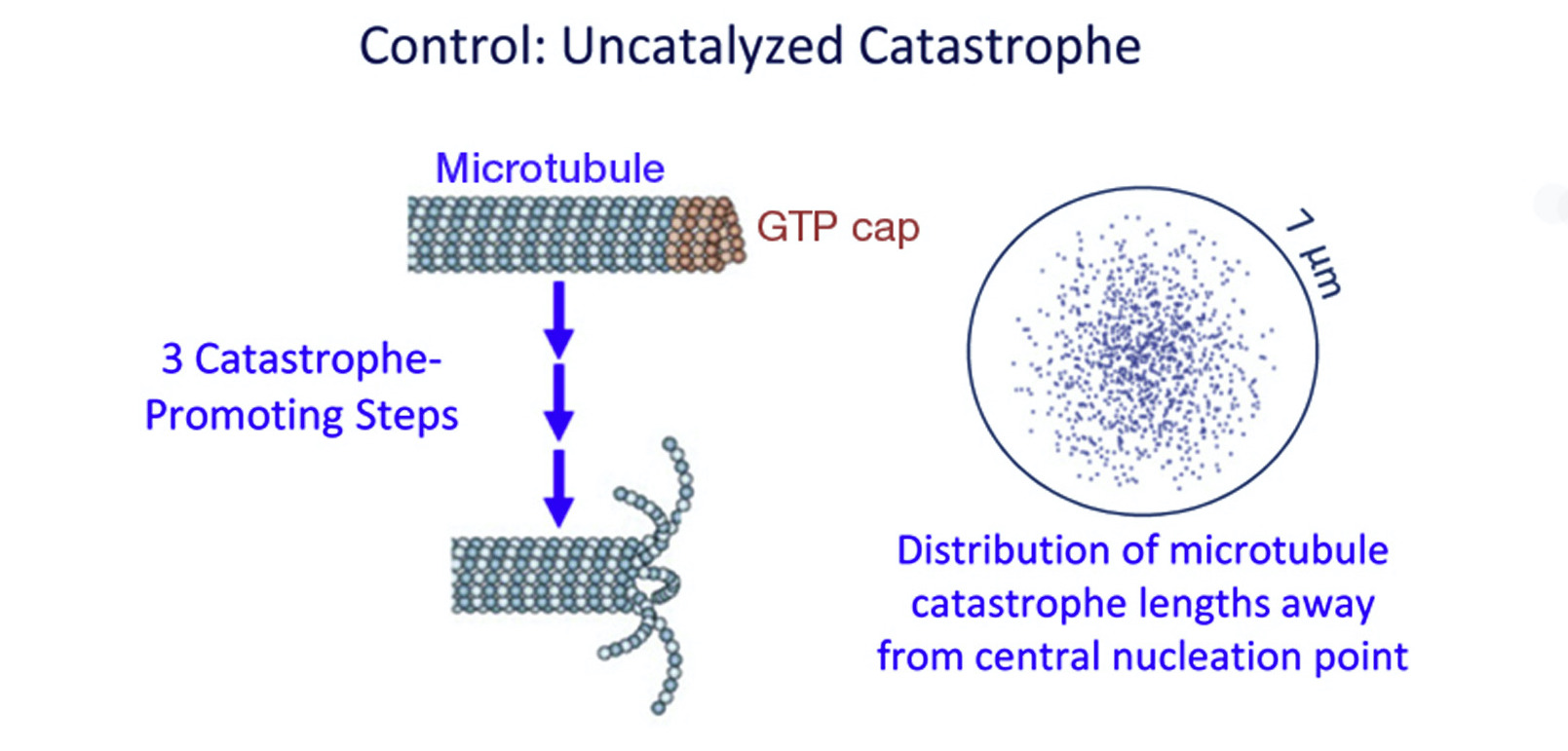
Figure 1. Microtubule catastrophe occurs when depolymerization is suddenly favored over tubulin polymerization, resulting in the loss of the GTP-bound tubulin cap. The paper by Garner and coworkers proposes a model in which catastrophe is a multi-step process. Source: Gardner et al., 2011
Experimental Methods
Gardner and coworkers monitored the dynamic instability of individual microtubules mainly via TIRF microscopy. Tubulin “seeds”, or stable foundations for microtubule growth, were labeled with rhodamine dye and fixed to a glass coverslip. GTP-bound tubulin, labeled with the fluorophore Alexa-488, was flowed over the coverslips and allowed to polymerize onto the immobilized tubulin seeds. Use of two distinct dyes enabled the researchers to distinctly observe and measure the polymerization and depolymerization events– the green tubulin could clearly be seen growing from the red tubulin seeds in real time. To confirm that the presence of the Alexa-488 dye did not interfere with the growth events, the authors performed a control experiment in which they monitored growth and depolymerization with unlabeled tubulin via differential interference contrast microscopy.
The following images were collected in a study by Varga et al., published in Nature in 2006. While not exactly representative of the images generated in this study, the images show how fluorescently labeled tubulin can be incorporated into microtubules through dynamic instability. This Nature study equipped Gardner and coworkers with the experimental methods used to generate the data that we’ll now explore!

Figure 2. A demonstration of tubulin incorporation into microtubles. Source: Varga et al., 2006
Statistical Methods Employed
We conduct statistical inference through a number of analyses, described here and in later sections. We demonstrate that there is no difference in time to microtubule catastrophe for labeled versus unlabeled tubulin through generation of bootstrap samples, calculation of statistical functionals and confidence intervals, and a null hypothesis significance test. To model the occurrence of microtubule catastrophe, we consider both the Gamma and Poisson distributions. We generate each of these models parameterized by data obtained by Gardner and coworkers, then conduct graphical and non-graphical model assessment to identify the more appropriate model.
Does tubulin labeling affect microtubule growth?
The authors’ TIRF experiment utilized Alexa-488 dye to image tubulin polymerization onto microtubules. To confirm that the dye doesn’t interfere with dynamic instability, the authors conducted a control experiment in which they monitor the time to catastrophe for both labeled and unlabeled tubulin. We evaluate the results of that experiment here.
Comparison of plug-in estimates
While evaluation by eye cannot replace more rigorous statistical inference, an eye test can be useful for initial assessment of the data. A plot of ECDFs for the time to catastrophe for labeled and unlabeled tubulin reveals that the two distributions are similar, however not identical (Figure 3). The 95% confidence regions generated in iqplot overlap significantly (Figure 3, shaded regions); however these observations are not enough to make conclusive statements regarding the similarity of the two distributions.
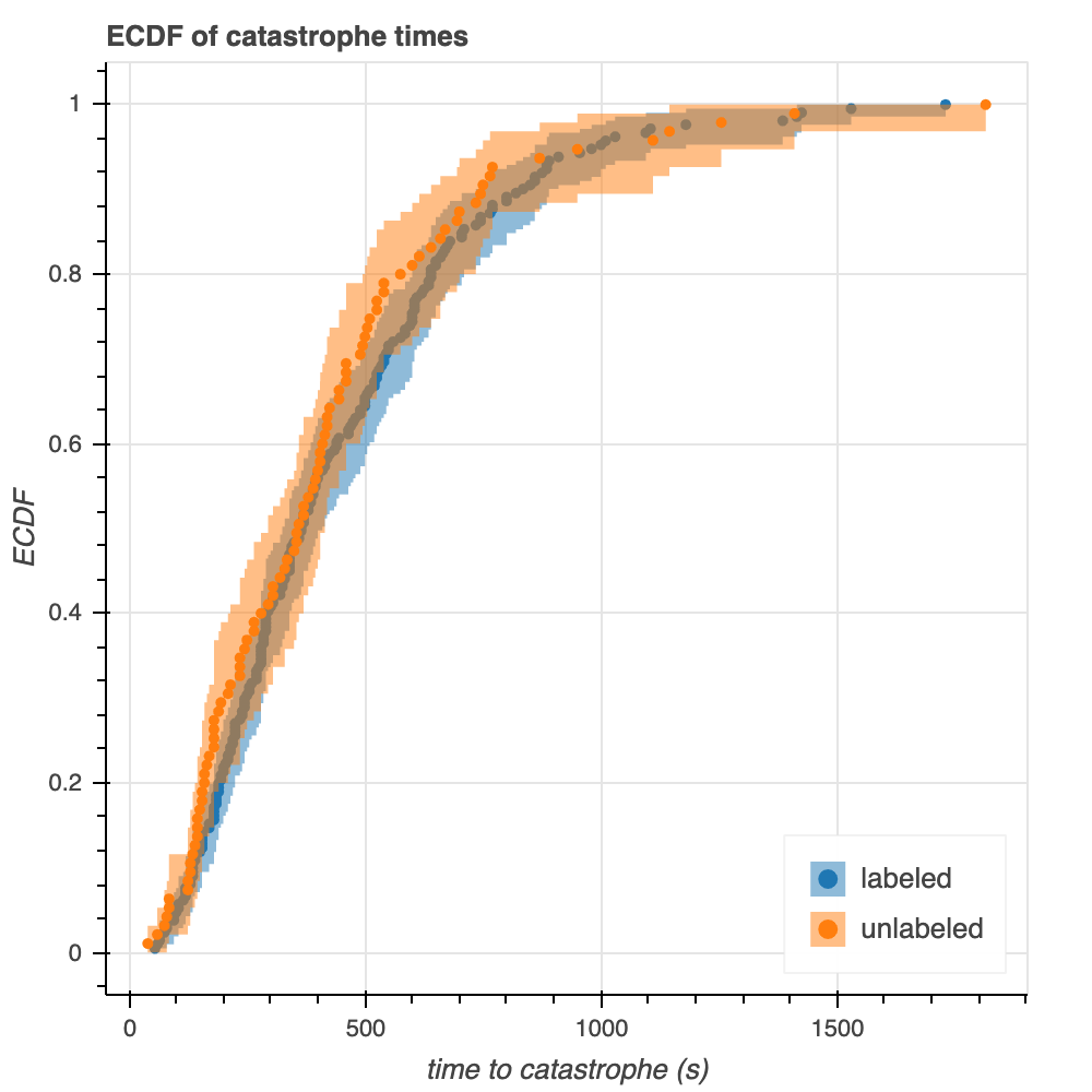
Figure 3. ECDFs of time to microtubule catastrophe for labeled and unlabeled tubulin. 95% confidence intervals are shown (shaded regions).
Calculating plug-in estimates, such as the mean, from the empirical distributions is another method of quick-checking the data for similarity but cannot provide any definite conclusions. These calculations show that the mean time to catastrophe is 440.7 seconds for labeled tubulin and 412.5 seconds for unlabeled tubulin. Once again, these values are similar, but in reality the mean of unlabeled tubulin is 93.6% the mean of labeled tubulin– the two are not identical.
Obtaining and comparing confidence intervals for the mean times to catastrophe provides more insight toward the similarity of this plug-in estimate than simply comparing two values does. Bootstrapping from the empirical data with a sample size of $n = 10000$, we generate 10,000 bootstrap replicates of the mean (Figure 4). Using these bootstrap replicates in our calculation of confidence intervals shows that the 95% confidence interval for the mean time to catastrophe for labeled tubulin is [401.87, 482.18] seconds, while this 95% confidence interval for unlabeled tubulin is [354.05, 476.32] seconds. These confidence intervals are similar, but the labeled confidence interval is narrower, and shifted towards longer values than, the unlabeled interval. Both of these phenomena are expected: there are more labeled datapoints, so we would expect a narrower confidence interval; additionally, as seen above, the mean of the labeled waiting times is above the mean of the unlabeled waiting times. As an aside, the two ECDFs of the mean times to catastrophe look like Normal distributions as the means of the samples obey the central limit theorerm. We confirm this observation through overlay of the ECDFs with theoretical CDFs of the normal distribution parameterized by the labeled and unlabeled tubulin data (Figure 5).
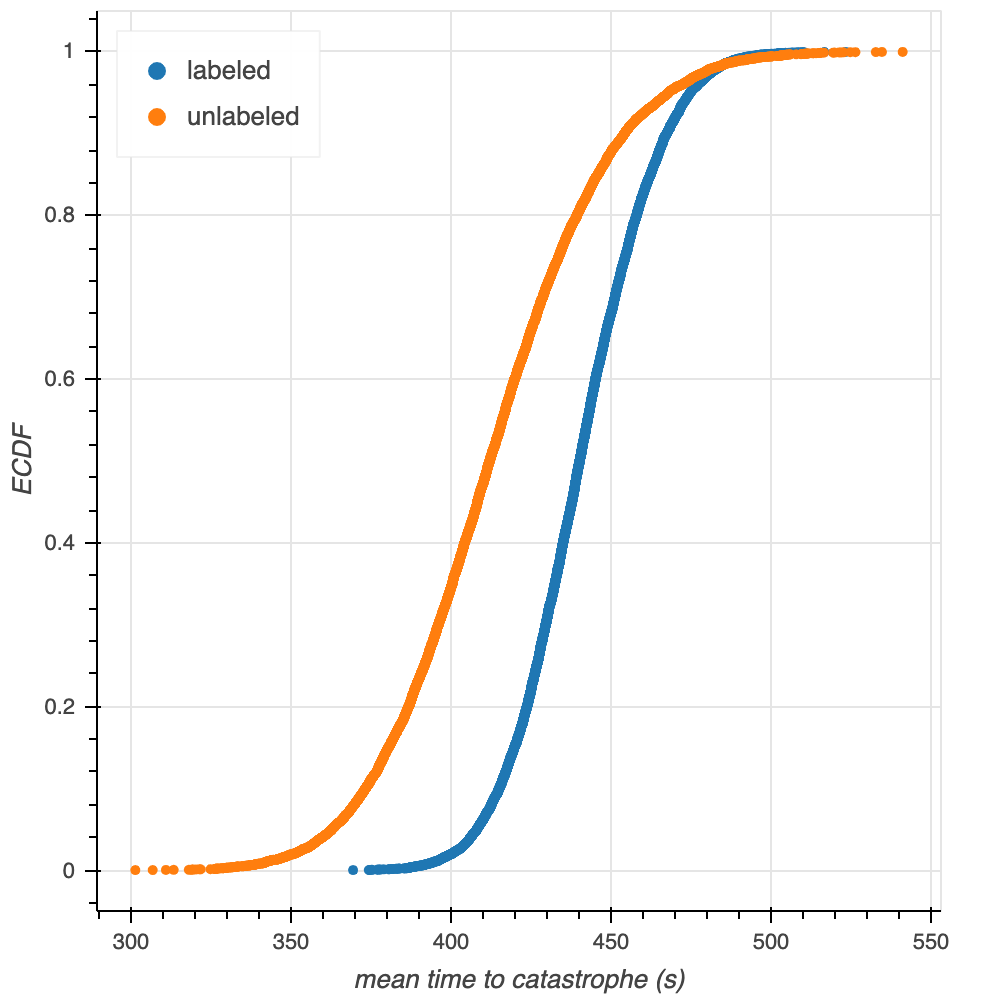
Figure 4. ECDFs of the bootstrapped mean times to catastrophe obtained for labeled and unlabeled tubulin. The two shapes look similar to what we might expect from the confidence intervals: the labeled ECDF is to the right of the unlabeled, and is steeper and narrower.
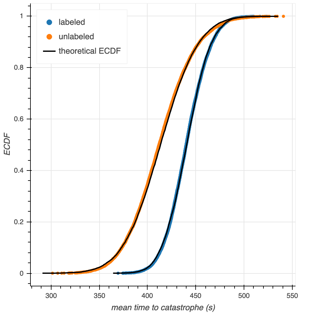
Figure 5. ECDFs of the bootstrapped mean times to catastrophe overlaid with theoretical CDFs of the Normal distribution parameterized by labeled and unlabeled tubulin data (black lines).
Construction of confidence intervals
We use theory to construct 95% confidence intervals for the ECDFs of the raw data (Figure 6). Specifically, we use the Dvoretzky-Kiefer-Wolfowitz Inequality (DKW) to identify upper and lower bounds between which lie the 95% confidence intervals. These upper and lower bounds correspond to the maximum distances between the ECDF and the generative CDF in the positive and negative directions.
There are some similarities and some differences between the confidence intervals from theory and those from bootstrapping (Figure 6). In both cases, the confidence intervals are wider for the unlabeled microtubules: this is expected, as the width of the confidence interval is inversely proportional to the root of the number of points. On the other hand, the confidence intervals are wider for the theoretical plot than the bootstrapped plot. This phenomenon could be attributed to the fact that these theoretical intervals come from upper bounds, which might be quite conservative.
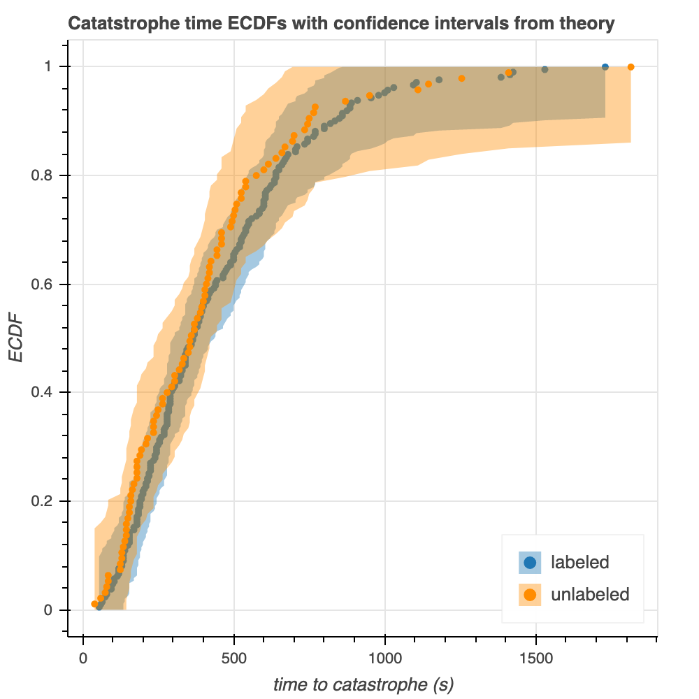
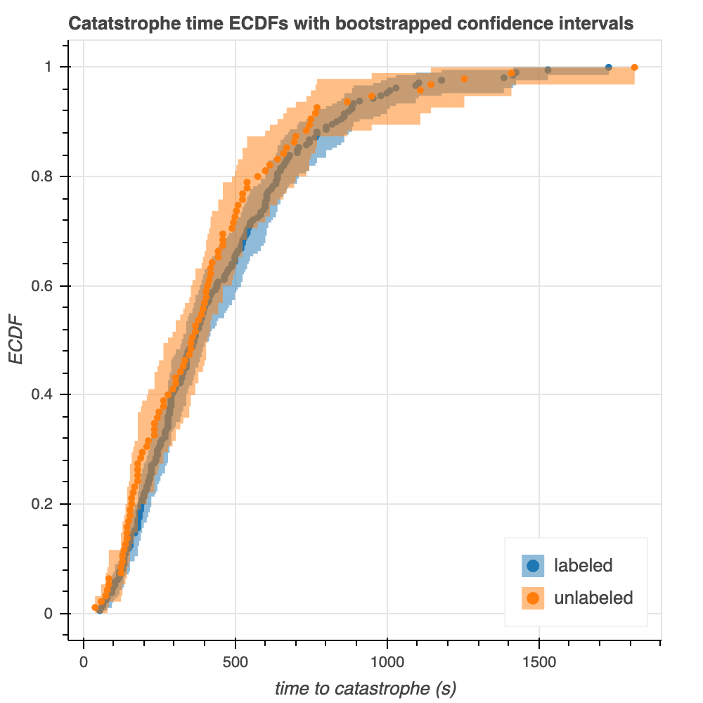
Figure 6. 95% confidence intervals calculated by theory (left) and bootstrapping from the empirical data (right).
Overall, there is very significant overlap of the theoretical confidence intervals for labeled an unlabeled tubulin, which supports the observations we have made thus far that the two are very similarly distributed.
Null hypothesis significance testing
We use NHST to test the hypothesis that the catastrophe time distributions are exactly the same for labeled and unlabeled microtubules. Given this hypothesis, we can use the permutation method: that is to say, under they hypothesis, labeled and unlabeled datapoints come from the exact same generative distribution, and so any difference in any statistical functional (e.g. mean, variance) between the two sets has arisen randomly when we sampled the underlying distribution to divide into these sets. Consequently, to test this hypothesis, we can combine all of the datapoints into a single set, and repeat the process of randomly dividing them into two samples with containing the same number of points as the experimental samples: under the hypothesis, this is how the experimental data were generated! We compute the statistical functionals on these ‘permuation’ samples, and see how often this is as extreme as it is for the experimental samples.
If we were to take a less conservative hypothesis, such that the sample means are the same but other functionals need not be the same, we would need to use a different approach to test it. (e.g. in this case, shifting the distributions to have the same mean, and seeing how often the bootstrapped mean difference is as large as the experimental value).
Given the hypothesis that the distributions are identical, if any statistical functional were found to be significantly different between the samples, we would reject the null hypothesis. We calculate the first (mean), second (variance), and third (skewness) moments as our statistical functionals, and find that the p-values are approximately 0.2, 0.6, and 0.9 for mean, variance, and skewness, respectively. For each of these statistical functionals, the p-value is above alpha = 0.001, and so we cannot use any of these as a reason to reject the null hypothesis.
Together, our findings from this section support our hypothesis that the distributions of time to catastrophe for labeled and unlabeled tubulin are similar. Until this point, we have not found any evidence to state that the two are significantly dissimilar. Therefore, we will assume that the Alexa-488 dye has no meaningful effect on dynamic instability, and from here on we will explore the data only considering labeled tubulin.
Is microtubule catastrophe a Gamma or Poisson distributed process?
In their paper, Garnder and coworkers assume that times to microtubule catastrophe are Gamma distributed. This is a fair assumption, considering data of theirs that suggest catastrophe is a multistep process. The Gamma distribution models the arrival times of a Poisson process in which all times are evenly spaced. As many biochemical reactions are Poisson processes, it is possible that microtubule catastrophe is Gamma distributed if each of the events leading to catastrophe occur at the same (or similar) rates.
We consider the possibility that the arrival times of the events leading to microtubule catastrophe are not evenly spaced, and that the data are better modeled using a Poisson distribution. For each distribution, we obtain parameter estimates through numerical optimization of maximum likelihood estimates using Powell’s method. These parameter estimates that we obtain ($\alpha$ and $\beta$ for the Gamma distribution and $\beta_1$ and $\beta_2$ for the Poisson distribution) are used to construct predictive ECDFs of microtubule catastrophe. We use a variety of methods, both graphical and non-graphical, to assess the similarity of the empirical data and the predictive ECDFs to determine which model is the better representation of microtubule catastrophe.
After generating predictive ECDFs, we overlay the empirical data with the 95% confidence intervals of these ECDFs (Figure 7). We see that the data falls within the predictive ECDF region of the Gamma distribution at almost all time points. The data falls largely outside of the predictive ECDF of the Poisson distribution– at times below ~400 seconds, the model overestimates the distribution, while at times greater than ~500 seconds, the model underestimates the distribution. From these plots alone, the Gamma distribution seems to be a better model for the data.
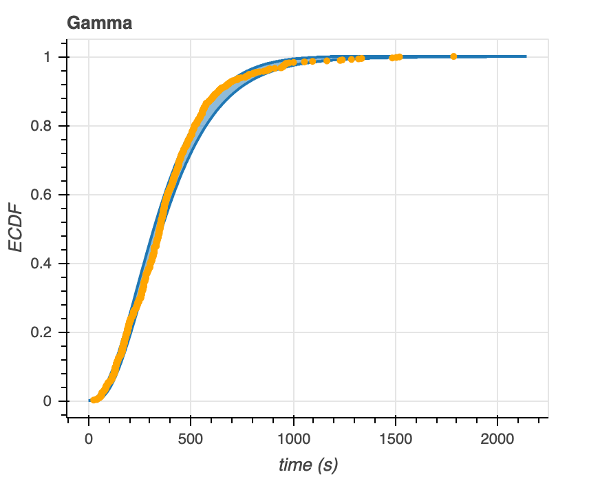
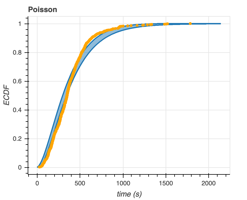
Figure 7. Predictive ECDFs for the Gamma (left) and Poisson (right) distributions overlaid with ECDFs of time to microtubule catastrophe.
We generate some Q-Q plots as another way to visualize how well the model distribution correlates to the data (Figure 8). For the Gamma distribution, the data fits within 95% of the Q-Q plots at times less than 1000 seconds. At times greater than 1000 seconds, the distribution falls outside of these intervals. However, from the data we see that there are relatively few microtubule catastrophe events happening at times greater than 1000 seconds– so the good fit of the data to our model at times below 1000 seconds is more important than the poor fit of the data to our model at times after 1000 seconds. With the Poisson distribution, we see almost completely the opposite. The data correlates with the model poorly at times below 1000 seconds yet shows better correlation at times above 1000 seconds. As stated above, the data contains few points corresponding to catastrophe times greater than 1000 seconds, so the Q-Q plot indicates that the Poisson distribution that we’ve defined does not fit the data very well.
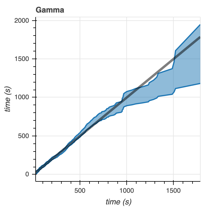
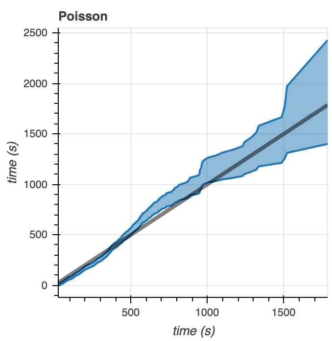
Figure 8. Q-Q plots comparing the model to the empirical data for the Gamma (left) and Poisson (right) distributions.
As a last method of graphical assessment, we make plots that show the difference between the predictive ECDF and the measured ECDF (Figure 9). The larger the ECDF difference (y-axis) in either the positive or negative direction, the larger the deviation from the median predictive EDCF, indicating a poor correlation between the model distribution and the actual data. Like we observe from the predictive ECDF plots above, we see that most of the experimental data falls within the 95% confidence intervals of the Gamma-distributed predictive ECDF (light blue shading). Much of the data falls outside of the 95% confidence intervals on the predictive ECDF of the Poisson distribution.
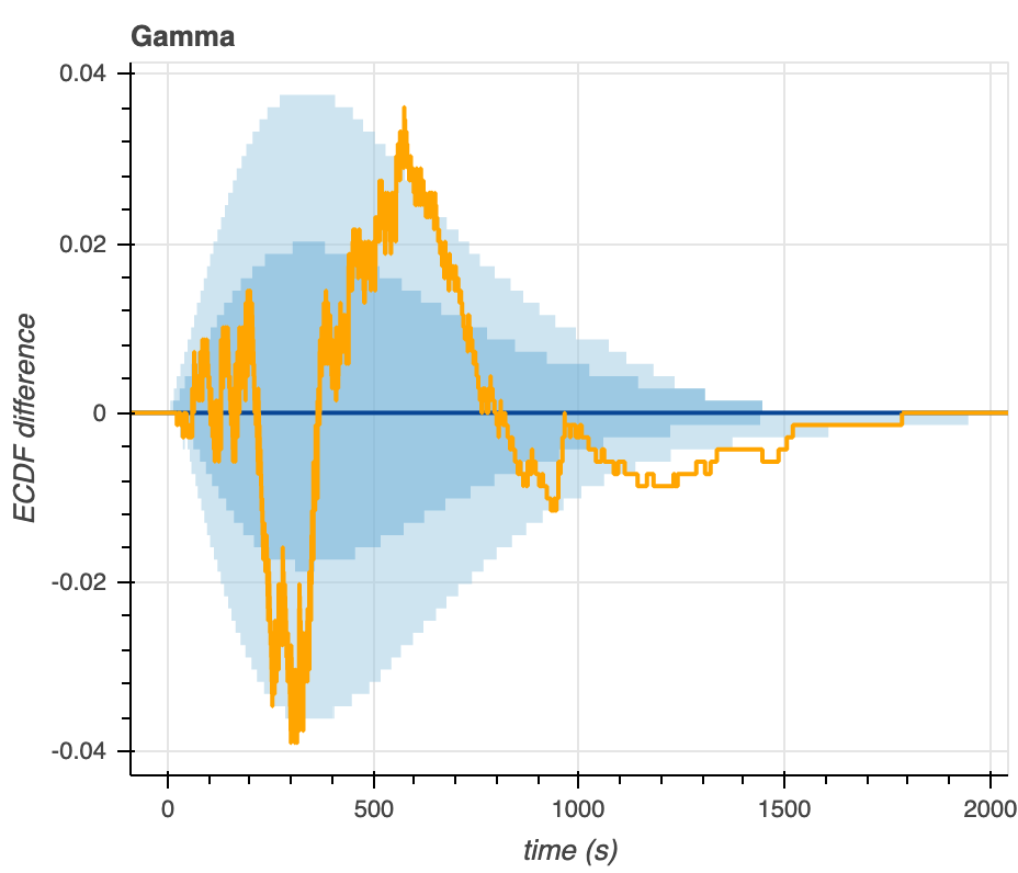
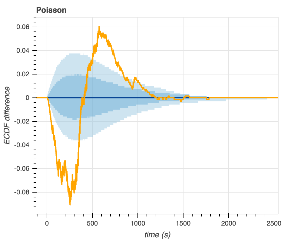
Figure 9. Visualization of the differences between the empirical and predictive ECDFs for the Gamma (left) and Poisson (right) distributions.
Overall, each of the graphical model assessments above give the same result and indicate that the Gamma distribution is a more accurate model of microtubule catastrophe. We next utilize some non-graphical methods of model assessment.
We next perform model comparison with the AIC. The AIC is a way of quantifying goodness-of-fit of the model while taking into account the complexity of, or number of parameters in, the model. Thus, when comparing two AICs corresponding to two models, the model with the smaller AIC is a better fit of the data (or closer to the actual generative distribution). The Gamma distribution has a smaller AIC compared to the Poisson distribution (Table 1), indicating that the true generative distribution is likely more Gamma-distributed than Poisson.
We can go one step further in our analysis by calculating the Akaike weights for each model compared to the other (Table 1). The Akaike weight of the Gamma model is approximately 1 since the Akaike weight of the Poisson model is so small (and AW_Gamma + AW_Poisson = 1). The Akaike weight of the Gamma model is loosely the probability that this model would better predict any new microtubule catastrophe data compared to the Poisson distribution. Therefore, because the Akaike weights indicate that the Gamma distribution would be a better model for new measurements, these results favor the Gamma distribution as a model for microtubule catastrophe.
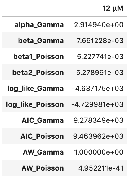
Table 1. Maximum likelihood estimates of the parameters, log-likelihoods, AICs, and Akaike weights for the Gamma and Poisson distributions at 12 $\mu$M tubulin concentration.
In summary, the AIC and Akaike weight calculations agree with the conclusion from the graphical model assessment that the Gamma distribution is the preferred model for microtubule catastrophe data.
What is the effect of tubulin on microtubule catastrophe time?
An ECDF of time to microtubule catastrophe at various tubulin concentrations shows that at increasing concentrations of tubulin, the time it takes for microtubule catastrophe to occur increases as well (Figure 10).
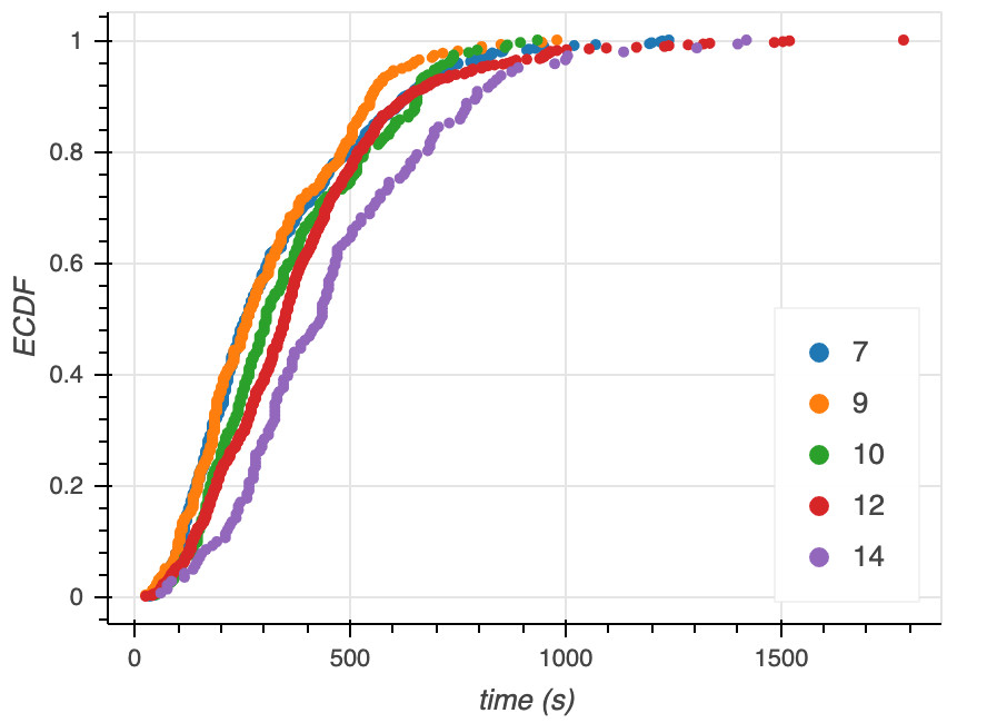
Figure 10. ECDFs of time to catastrophe at various tubulin concentrations (legend).
We can confirm these initial observations through comparison of parameter estimates at each tubulin concentration (Table 2, Figure 11). As we demonstrated above, the Gamma distribution seems to be the better model of microtubule catastrophe, thus we compare the $\alpha$ and $\beta$ parameter estimates for all concentrations. Since the mean of Gamma-distributed data is equal to $\alpha/\beta$, we also calculate and compare this parameter estimate.
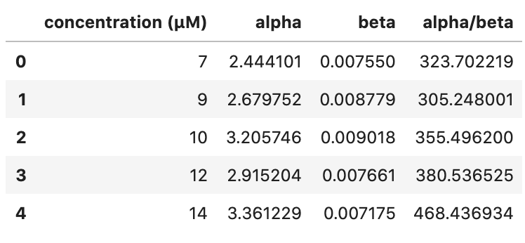
Table 2. Parameters $\alpha$, $\beta$, and $\alpha/\beta$ of the Gamma distribution for various tubulin concentrations.
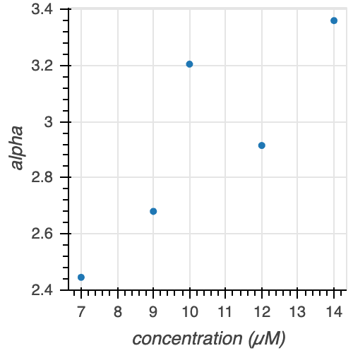
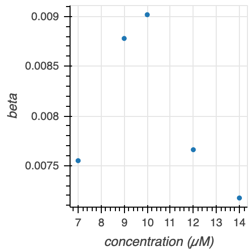
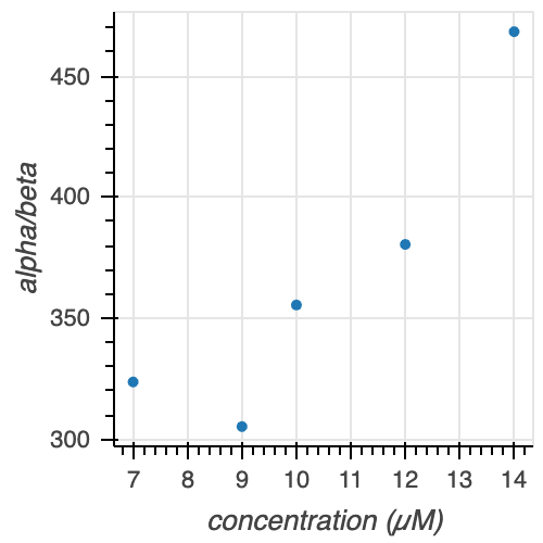
Figure 11. Gamma parameters $\alpha$, $\beta$, and $\alpha/\beta$ at various tubulin concentrations.
There is no clear trend for either the $\alpha$ or $\beta$ parameter estimates with increasing tubulin concentration. However, we see that $\alpha / \beta$ increases with increasing tubulin concentration (with the exception of 7 and 9 uM tubulin, which appear to be very similarly distributed looking back at the ECDFs in Figure 10). Thus, we can conclude that with increasing tubulin concentration, the average time to catastrophe increases.
This conclusion makes sense within the context of microtubule catastrophe. As stated in the paper, microtubules (tubulin polymers) are dynamic macromolecules that undergo alternating periods of growth and shrinking. Catastrophe occurs when microtubule shortening is suddenly favored over growth. A longer time to catastrophe indicates the microtubules withstand the alternating growth and shortening pattern for a greater period of time.
We assume that increasing the concentration of tubulin favors microtubule growth. In a chemical reaction under equilibrium, increasing the concentration of reactants shifts the equilibrium such that the forward reaction to product is favored. We apply this logic to the case of microtubules: increasing the tubulin, or reactant, concentration should favor the forward reaction of microtubule polymerization rather than the reverse shortening reaction. Thus, we conclude that increasing the concentration of tubulin presumably promotes microtubule growth and delays the turning point at which shortening is favored, resulting in a greater mean time to catastrophe.
Summary
In our analysis of data generated by Gardner and coworkers, we confirm their findings that microtubule catastrophe is best modeled as a Gamma-distributed process with all catastrophe events occurring at the same rate. We find that in their experiment, labeling of tubulin has no appreciable impact on the process of dynamic instability. Finally, we see that microtubule catastrophe is delayed by addition of tubulin, presumably due to the presence of tubulin prolonging the alternating period of microtubule growth and shortening.
A mathematical aside on the Poisson distribution
We consider a Poisson process with two different rates to arrival, $\beta_1$ and $\beta_2$. The formula of the Poisson distribution is \begin{align}
f(t_i) = \beta_i e^{-\beta_i t_i}
\end{align} We can explore what happens when we incorporate the two rates into the formula.
Let $t_1 =$ time it takes for step 1
Let $t_2 =$ time it takes for step 2 (after step 1)
Therefore, we have
\begin{align}
f(t_1) = \beta_1 e^{-\beta_1 t_1}
\end{align}
And
\begin{align}
f(t_2) = \beta_2 e^{-\beta_2 t_2}
\end{align}
$t = t_1 + t_2$, therefore $t_2 = t - t_1$. Combining the distributions to model two consecutive events $t_1$ and $t_2$ gives:
\begin{align}
f(t_1, t_2) = \beta_1 \beta_2 e^{-\beta_1 t_1} e^{-\beta_2 t_2}
\end{align}
This is true because $f(t_1)$ and $f(t_2)$ are independent. Applying the substitution for $t_2$ gives:
\begin{align}
f(t_1, t) = \left|\frac{\mathrm{d} t_1}{\mathrm{d}t} \right|\beta_1 \beta_2 e^{-\beta_1 t_1} e^{-\beta_2 (t-t_1)}
\end{align}
$ \left|\frac{\mathrm{d} t_1}{\mathrm{d}t} \right| = 1$, therefore
\begin{align}
f(t_1, t) = \beta_1 \beta_2 e^{-\beta_1 t_1} e^{-\beta_2 (t-t_1)}
\end{align}
Marginalizing to eliminate the $t_1$ term gives:
(Note: the integral is evaluated from $0$ to $t$ as $t$ is the maximum value of $t_1$)
\begin{align}
f(t) &= \int_0^t \mathrm{d}t_1 \, f(t, t_1)
\end{align} \begin{align}
& = \int_0^t \mathrm{d}t_1 \, \beta_1 \beta_2 e^{-\beta_1 t_1} e^{-\beta_2 (t-t_1)}
\end{align} \begin{align}
& = \left [ \frac{1}{-\beta_1 - (-\beta_2)} \, \beta_1 \beta_2 e^{-\beta_1 t_1} e^{-\beta_2 (t-t_1)} \, \right]_0^t
\end{align} \begin{align}
& = \left ( \frac{1}{\beta_2 - \beta_1} \right )[\beta_1\beta_2 e^{-\beta_1 t} e^{-\beta_2 (0)}] - [\beta_1\beta_2 e^{-\beta_1 (0)} e^{-\beta_2 (t-0)}]
\end{align} \begin{align}
& = \left ( \frac{1}{\beta_2 - \beta_1} \right )[\beta_1\beta_2 e^{-\beta_1 t} \, (1)] - [\beta_1\beta_2 \, (1) \, e^{-\beta_2 t}]
\end{align} \begin{align}
& = \left ( \frac{1}{\beta_2 - \beta_1} \right )[\beta_1\beta_2 e^{-\beta_1 t}] - [\beta_1\beta_2 e^{-\beta_2 t}]
\end{align} \begin{align}
& = \left ( \frac{1}{\beta_2 - \beta_1} \right )(\beta_1\beta_2)(e^{-\beta_1 t} - e^{-\beta_2 t})
\end{align} \begin{align}
& = \left ( \frac{\beta_1\beta_2}{\beta_2 - \beta_1} \right )(e^{-\beta_1 t} - e^{-\beta_2 t})
\end{align}
Therefore
\begin{align}
f(t; \beta_1, \beta_2) = \left ( \frac{\beta_1\beta_2}{\beta_2 - \beta_1} \right )(e^{-\beta_1 t} - e^{-\beta_2 t})
\end{align}
In the case of the limit where $\beta_1$ approaches $\beta_2 = \beta$, the equation becomes
\begin{align}
f(t; \beta) = \beta^2 t e^{-\beta t}
\end{align}
This equation corresponds to the PDF of the Gamma distribution when $\alpha = 2$!
Acknowledgements
We would like to thank Gardner, coworkers, and all other scientists who generously shared their data with us over the course of the semester; the TAs for their hard work in making BE/Bi103a a success; Griffin Chure for his website template and general wisdom; and of course, Justin Bois, for his constant effort, enthusiasm, and dedication to his students.
Data Set Downloads
Raw Data, Labeled vs. Unlabeled Tubulin
Raw Data, Varying Tubulin Concentrations
References
Cooper GM. The Cell: A Molecular Approach. 2nd edition. Sunderland (MA): Sinauer Associates; 2000. Microtubules. Available from https://www.ncbi.nlm.nih.gov/books/NBK9932/
Gardner MK, Zanic M, Gell C, Bormuth V, Howard J. Depolymerizing kinesins Kip3 and MCAK shape cellular microtubule architecture by differential control of catastrophe. Cell. 2011 Nov 23;147(5):1092-103. doi: 10.1016/j.cell.2011.10.037. PMID: 22118464.
Varga, V., Helenius, J., Tanaka, K. et al. Yeast kinesin-8 depolymerizes microtubules in a length-dependent manner. Nat Cell Biol 8, 957–962 (2006). https://doi.org/10.1038/ncb1462